In this blog post, I'm going to explain how the gSpan algorithm works for mining frequent patterns in graphs. If you haven't already read my introductory post on this subject, please click HERE to read the post that lays the foundation for what will be described in this post.
Getting Started
To explain how this algorithm works, we're going to work through a simplified data set so that we can see each step and understand what is going on. Suppose that you have 5 graphs that look like this

Don't get confused by the greek characters here. I used random symbols to show that this method can be used for any type of graph (chemicals, internet web diagrams, etc.) even something completely made up like what I did above. The first thing we need to do with this graph data set is count how many vertices and edges we have of each type. I count 7 alpha(α) vertices, 8 beta(β) vertices, and 14 lambda(λ) vertices. There are 15 edges that are solid blue, 13 that are double red, and 8 that are dotted green. Now that we have these counts we need to order the original labels for vertices and edges into a code that will help us prioritize our search later. To do this we create a code that starts with the vertices and edges with the highest counts and then descends like this
.jpg)
We could have used numbers instead of letters here, it doesn't really matter as long as you can keep track of the symbols' order based on frequency. If you relabel the graphs with this order you get something like this
 You can see that the vertex labels now have A, B, C and each edge is labelled a, b, or c to match the new label legend we created.
Finding Frequent Edges
For this example we will assume that we have a minimum support frequency of 3 (i.e. 3 of the 5 graphs have to have the pattern for us to consider it important). We start by looking at individual edges (e.g. A,b,A) and see if they meet this minimum support threshold. I'll start by looking at the first graph at the top. There is an edge that is (B,a,C) and I need to count how many of the graphs have an edge like this. I can find it in the 1st graph, 2nd graph, 3rd graph, and 4th graph so it has support of 4; we'll keep that one. Also notice that I had the option of writing that edge as (C,a,B) as well, but chose to write it with B as the starting vertex, because of the order we established above. We move on a little and check (A,a,C) and find that it can only be found in the first graph; it gets dropped. We check (A,c,C) and find it in the first 4 graphs as well; keep it. If we continue going through all of the graphs being careful not to repeat any edge definitions we'll get a list of frequent single edges that looks like this

You can see that we only have 3 edges that are frequent (this will simplify our lives in this example greatly). We need to sort the edges that are still frequent in DFS lexicographic order (See prior blog post for explanation of this). After sorting we end up with this list of edges to consider going forward
.jpg)
Pay attention to the fact that I added the "0,1" to the beginning of these edge definitions. These are the starting and ending points of the edges. We'll "grow" the rest of the frequent sub-graphs from these edges in a way similar to the method described in my prior blog post on this subject.
gSpan starts with the "minimum" edge, in this case (0,1,A,b,B), and then tries to grow that edge as far as it can while looking for frequent sub-graphs. Once we can't find any larger frequent sub-graphs that include that first edge, then we move on to the 2nd edge in the list above (0,1,A,c,C) and grow it looking for frequent sub-graphs. One of the advantages of this is that we won't have to consider sub-graphs that include the first edge (0,1,A,b,B) once we've moved on to our 2nd edge because all of the sub-graphs with the first edge will have already been explored. If you didn't follow that logic, it's OK; you'll see what I mean as we continue the example.
You might notice that the last graph in our set of graphs doesn't have any edges that are frequent. When we're starting with edge (A,b,B) we keep track of which graphs have that edge present. In our example that's graphs 1, 2, 3, & 4. Now that we have that "recorded" we start the growth from (0,1,A,b,B) by generating all of the potential children off of the 'B' vertex.
Growing from the 1st Edge
Before we grow our first edge, you need to understand how gSpan prioritizes growth. Let's assume that we have a generic subgraph that looks like this already (don't worry about how we got it yet, it will be come clear in a second)

I have removed the colors and labels from the diagram above to explain how gSpan grows without confusing you with labels. The numbers represent the order the vertices were added. If you are at this point in the algorithm, you will try to grow this graph in the following order of priority.

So the first priority is always to link the current end vertex back to the first vertex (the one labelled 0). If that's not possible, we see if we can link it back to the 2nd vertex (the one labelled 1). If we had a bigger sub-graph, we would continue trying to link to the 3rd, 4th, etc. if it's possible. If none of those are possible then our next (3rd) priority is to grow from the vertex we're at (labelled 4 above), and grow the chain longer. If that doesn't work, we go back to the most recent fork, take another step back and then try to grow from there (see how 5 is growing from vertex labelled 1 in the 4th priority). If that doesn't work, then we take another step up the chain and try to grow from there (5th example above). The 4th and 5th examples above also generalize for longer chains. If there were several vertices above the closest fork in the chain, you would progressively try to grow off of each of those vertices until you get back to the root (vertex labelled '0').
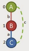
With that understanding in mind, we can finally start growing from our first edge. Our first edge is (0,1,A,b,B). If we look at the priority explanation above, we can tell that the 1st and 2nd growth priorities are not really options, so we take the 3rd priority and try to grow from vertex 1, or the B vertex in our example. Since we only have 2 frequent edges that have 'B' vertices in them our two options are as follows:
Option 1 Option 2
(0,1,A,b,B) (0,1,A,b,B)
(1,2,B,b,A) (1,2,B,a,C)
Now we are going to check for support of these 2 options. We only need to look in the graphs that we determined contain the frequent edges as described earlier. When we look for Option 1 we find it in the following graphs left that we're considering:

Notice that we can find the first option in 3 different places in the first graph, but we can't find it in any of the other graphs, so the support is only 1. That's a dead end, so we check option 2
.jpg)
You can see that we can find this pattern in multiple places in all of the 4 graphs we have left (I didn't show all of the places it is found in the first graph). The support for this sub-graph is 4 so it's a keeper. Also, all 4 graphs we looked at have this sub-graph present so we keep those too. That ends that round of edge growth so we take option 2 from above and try to grow from it. Remembering the priorities of growth, we know we need to try to connect the last vertex (2 or 'C' in our example) to the root (0 or 'A' in our example) if we can. If we look at the list of frequent edges to choose from, we see an edge that is (A,c,C) which could be written as (2,0,C,c,A). This would make the connection we need. None of the other frequent edges meet this criteria, so we check to see if (0,1,A,b,B); (1,2,B,a,C); (2,0,C,c,A) is frequent


As it turns out, this 4 edge pattern can only be found in 2 of the 4 graphs we have left so that doesn't work. Now we'll check if (2,3,C,c,A) works out.

Nope, that's only in the first graph so it's not frequent either. Since neither of these worked out, we need to go to our next priority (4th) which is growing from the vertex a step up from the last attempted branch. When you look at the sub-graph we've grown so far you can tell we need to try to grow from 'B' now. That being said, we take a look at our options for frequent edges that contain 'B' vertices and we see that we should try to add (B,a,C) or (B,b,A). Here's what trying to add (B,a,C) looks like in this scenario


As it turns out, we CAN find this sub-graph in 3 of the 4 graphs we have left so that's a keeper. At this point in time I want you to notice that I am going to ignore the other edge that could grow from 'B' until later. This is because gSpan is a depth first algorithm, so once you get success you try to go deeper. When we hit a dead end, we will come back to all of these straggling options to see if they actually work. If you're familiar with computer programming, this type of algorithm is implemented with recursion. Our next step based on our priority rules is going to be to try to link our vertex 3 ('C') to the root, or the 'A'. Again the only frequent edge we can choose from to do this is (C,c,A). This option would look like this

At this point, remember that the last sub-graph that we found that was frequent could only be found in the first 3 graphs in our set, so now we only have to look for this new graph in those three graphs

This only exists in one of our graphs, so we go to our next growth priority. Since there is already a link between our 'C' at vertex 3 and the 'B' and vertex 1, the 2nd priority isn't an option, so we try to grow/extend from the 'C' at vertex 3 again. We can either add (C,a,B) or (C,c,A). Adding (C,a,B) would look like this

If we look in the 3 graphs we have left we find this

That's a dead end because we only have 1 graph with this 5 edge sub-graph. We back up and try adding (C,c,A) instead. I'm not going to do the visuals for this, but it can't be found in any of the graphs we have left either. Since we hit a dead end again here, we go to to our 5th priority growth option: growing from the root again. If we try to grow from the root 'A' we can either use (A,b,B) or (A,c,C). Starting with (A,b,B) we would get a sub-graph that looks like this

This can't be found in any of our graphs, so we try adding (A,c,C) as our last ditch effort

This can't be found either, so we have reached the end of this depth first search. Now we need to go back and take care of the straggler options that we didn't pursue because we were going for depth first. The last straggling option we left was when we were considering adding (B,b,A) to vertex 1.

Remember, at that point in time, we were still looking at 4 of the 5 original graphs so when we look for this sub-graph in those 4 graphs this is what we find.

We only find it in one graph, so that turns into a dead end too.
This Section Until "2nd Edge (A,c,C)" is a Correction (Thanks to Elife Öztürk)
If we look back further in our algorithm we find that we also haven't checked all of the growth priorities off of the first frequent edge (0,1,A,b,B). Our first growth came from using the 3rd priority growth strategy, but we haven't checked the 4th/5th priority grown strategies there yet. If we do, we can see that it might be possible to make a link like (0,1,A,b,B) and (0,2,A,c,C). Let's see if we can find that in the graphs

We can see that in all four of our remaining graphs so we'll keep this sub-graph.
Our first priority for growth on this sub-graph would be to connect back to the root, but we don't have any double bonds (sorry for the chemistry reference) in our example so that won't work. The 2nd priority is also impossible, so let's check the 3rd. Can we grow an edge off of the C node? Our 2 options would be (2,3,C,a,B) and (2,3,C,c,A). Adding (2,3,C,a,B) looks like this.

When we search through the graphs, we find this in 2 places

Notice that I'm not counting the instances in the 2nd and 3rd graphs. This is because the only way you can get find this subgraph in those graphs is to wrap the graph such that the 1 B node is the same as the 3 B node. The reason why we number the nodes is to make sure they're unique, plus we already found the sub-graph that creates that ABC triangle previously...thus the beauty of the algorithm :). Since there are only 2 graphs with this sub-graph, the minimum support of 3 is not met.
So now let's check for the other growth option (2,3,C,c,A)

That can only be found in one of the graphs

So now we've exhausted our growth options off of the first edge (A,b,B).
2nd Edge (A,c,C)
Before you go crazy thinking that the other 2 edges we need to check will take just as long, let me tell you that we have already done WAY more than half of the work on this problem. Now that we have exhaustively checked all of the graphs for frequent sub-graphs that contain the edge (A,b,B), we can trim down our search space significantly. What I mean is we can delete edges in graphs that contain (A,b,B) and only look for frequent patterns in what is left. If we do this, we get 4 graphs (remember we already got rid of graph 5 because it contained no frequent edges) that look like this.

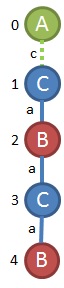
These graphs are much simpler. I also wanted to point out that I removed any edges from these graphs that were not frequent. We could (should) have done this earlier when we were doing our search on the first edge, but I didn't want to complicate things at that time. Now, much like last time, we start with edge (0,1,A,c,C) and try to grow from 'C'. We can either use (1,2,C,a,B) or (1,2,C,c,A). If we add (1,2,C,a,B) we can find that sub-graph in the following places

All 4 graphs have this sub-graphs, so it's a keeper and we'll go with it (remember we haven't checked adding (1,2,C,c,A) yet. The next step is to try to grow from the last vertex back to the root. If we did this we would have to use the edge (B,b,A), but that edge has been removed from all of our graphs because we have already mined all of the frequent sub-graphs with (A,b,B) in them. So, our only other growth option is to try to extend the chain from 'B'. The only option left to grow from 'B' is (B,a,C) because (B,b,A) has already been checked. So we get a sub-graph like this.

This can be found in the following graphs

That's 3 out of the 4 graphs, which meets our support requirement so we'll keep it. Our first growth priority from here is to link node 3 ('C') back to the root. That would be adding a (3,0,C,_,A) link. The only link possible for this in our data set is (3,0,C,c,A) which would give us this subgraph to look for

The only place this subgraph is found is in our 2nd example:
 So, that's a dead end. If we back up, our next growth priority would be to connect the C at node 3 back to the C at node 1. A quick look at the graphs we have tells me that's not going to work. The next priority after that is to add another node after node 3. We could look for a subgraph with C,a,B added to the end that looks like this.
However, that subgraph is only found here:

So, we back up again and try our 4th priority, which is growing a link off of the B at node 2. A quick look at the graphs above show that won't work. Lastly, we'll try to grow further up the graph, like a new node coming off the C at node 2 or a new node off the A at node 0. There's a couple options for growth off of node 2, but I can tell it's only supported by our first graph. There are no additional options for growth from the root node 'A'. so we're done exploring this graph branch.
Now we need to step back to when we had the graph (0,1,A,c,C), (1,2,C,a,B) and try to grow again from there. The last priority for growth for this subgraph is to grow from the root. The only way we can grow from the root is to add (A,c,c), which would look like this.
 Checking the four graphs we have left, we only find this sub-graph in our 2nd graph

Since this is only found in one place, it's a dead end and we need to backtrack to other options we didn't pursue earlier. We only had one of those when we were adding our 2nd edge to (A,c,C). So when we go back and try to add (1,2,C,c,A) to (0,1,A,c,C) we look at our graphs and find that it is only present in 2 of our graphs

As it turns out these are all of our options starting with edge (A,c,C). See, I told you the 2nd edge would go faster than the first.
3rd Edge (B,a,C)
Now we have to check the last of our frequent edges to see if there is any way that we can grow a frequent sub-graph with just this edge. Let's start by removing all of the (A,c,C) edges from our graphs to see what we're left with.

I could go through all of the same procedure I have been using for these remaining graphs, but it gets so simple at this point that there really isn't a reason to. If you're using a program runing the gSpan algorithm, it will be disciplined and do the whole search though. From what is left, we can see that (0,1,B,a,C); (0,2,B,a,C) is frequent, but anything larger doesn't work out. We hit our last dead end and now we can report all of the sub-graphs that we found that were frequent.

I have them organized by the edge they were grown from. The last thing we have to do is translate our DFS codes back to the original symbols. This is easy enough and the user would get an output like this.

That's all there is to it. I know that this post got a little long, but for me, being able to see the whole problem worked out helps me learn a TON. I hope it helps somebody else out there too. I did gloss over some details of the programming, etc. but this is essentially what's happening in gSpan. Let me know if you have any additional questions.
Getting Started
To explain how this algorithm works, we're going to work through a simplified data set so that we can see each step and understand what is going on. Suppose that you have 5 graphs that look like this
Don't get confused by the greek characters here. I used random symbols to show that this method can be used for any type of graph (chemicals, internet web diagrams, etc.) even something completely made up like what I did above. The first thing we need to do with this graph data set is count how many vertices and edges we have of each type. I count 7 alpha(α) vertices, 8 beta(β) vertices, and 14 lambda(λ) vertices. There are 15 edges that are solid blue, 13 that are double red, and 8 that are dotted green. Now that we have these counts we need to order the original labels for vertices and edges into a code that will help us prioritize our search later. To do this we create a code that starts with the vertices and edges with the highest counts and then descends like this
We could have used numbers instead of letters here, it doesn't really matter as long as you can keep track of the symbols' order based on frequency. If you relabel the graphs with this order you get something like this
Finding Frequent Edges
For this example we will assume that we have a minimum support frequency of 3 (i.e. 3 of the 5 graphs have to have the pattern for us to consider it important). We start by looking at individual edges (e.g. A,b,A) and see if they meet this minimum support threshold. I'll start by looking at the first graph at the top. There is an edge that is (B,a,C) and I need to count how many of the graphs have an edge like this. I can find it in the 1st graph, 2nd graph, 3rd graph, and 4th graph so it has support of 4; we'll keep that one. Also notice that I had the option of writing that edge as (C,a,B) as well, but chose to write it with B as the starting vertex, because of the order we established above. We move on a little and check (A,a,C) and find that it can only be found in the first graph; it gets dropped. We check (A,c,C) and find it in the first 4 graphs as well; keep it. If we continue going through all of the graphs being careful not to repeat any edge definitions we'll get a list of frequent single edges that looks like this
You can see that we only have 3 edges that are frequent (this will simplify our lives in this example greatly). We need to sort the edges that are still frequent in DFS lexicographic order (See prior blog post for explanation of this). After sorting we end up with this list of edges to consider going forward
Pay attention to the fact that I added the "0,1" to the beginning of these edge definitions. These are the starting and ending points of the edges. We'll "grow" the rest of the frequent sub-graphs from these edges in a way similar to the method described in my prior blog post on this subject.
gSpan starts with the "minimum" edge, in this case (0,1,A,b,B), and then tries to grow that edge as far as it can while looking for frequent sub-graphs. Once we can't find any larger frequent sub-graphs that include that first edge, then we move on to the 2nd edge in the list above (0,1,A,c,C) and grow it looking for frequent sub-graphs. One of the advantages of this is that we won't have to consider sub-graphs that include the first edge (0,1,A,b,B) once we've moved on to our 2nd edge because all of the sub-graphs with the first edge will have already been explored. If you didn't follow that logic, it's OK; you'll see what I mean as we continue the example.
You might notice that the last graph in our set of graphs doesn't have any edges that are frequent. When we're starting with edge (A,b,B) we keep track of which graphs have that edge present. In our example that's graphs 1, 2, 3, & 4. Now that we have that "recorded" we start the growth from (0,1,A,b,B) by generating all of the potential children off of the 'B' vertex.
Growing from the 1st Edge
Before we grow our first edge, you need to understand how gSpan prioritizes growth. Let's assume that we have a generic subgraph that looks like this already (don't worry about how we got it yet, it will be come clear in a second)
I have removed the colors and labels from the diagram above to explain how gSpan grows without confusing you with labels. The numbers represent the order the vertices were added. If you are at this point in the algorithm, you will try to grow this graph in the following order of priority.
So the first priority is always to link the current end vertex back to the first vertex (the one labelled 0). If that's not possible, we see if we can link it back to the 2nd vertex (the one labelled 1). If we had a bigger sub-graph, we would continue trying to link to the 3rd, 4th, etc. if it's possible. If none of those are possible then our next (3rd) priority is to grow from the vertex we're at (labelled 4 above), and grow the chain longer. If that doesn't work, we go back to the most recent fork, take another step back and then try to grow from there (see how 5 is growing from vertex labelled 1 in the 4th priority). If that doesn't work, then we take another step up the chain and try to grow from there (5th example above). The 4th and 5th examples above also generalize for longer chains. If there were several vertices above the closest fork in the chain, you would progressively try to grow off of each of those vertices until you get back to the root (vertex labelled '0').
With that understanding in mind, we can finally start growing from our first edge. Our first edge is (0,1,A,b,B). If we look at the priority explanation above, we can tell that the 1st and 2nd growth priorities are not really options, so we take the 3rd priority and try to grow from vertex 1, or the B vertex in our example. Since we only have 2 frequent edges that have 'B' vertices in them our two options are as follows:
Option 1 Option 2
(0,1,A,b,B) (0,1,A,b,B)
(1,2,B,b,A) (1,2,B,a,C)
Now we are going to check for support of these 2 options. We only need to look in the graphs that we determined contain the frequent edges as described earlier. When we look for Option 1 we find it in the following graphs left that we're considering:
Notice that we can find the first option in 3 different places in the first graph, but we can't find it in any of the other graphs, so the support is only 1. That's a dead end, so we check option 2
You can see that we can find this pattern in multiple places in all of the 4 graphs we have left (I didn't show all of the places it is found in the first graph). The support for this sub-graph is 4 so it's a keeper. Also, all 4 graphs we looked at have this sub-graph present so we keep those too. That ends that round of edge growth so we take option 2 from above and try to grow from it. Remembering the priorities of growth, we know we need to try to connect the last vertex (2 or 'C' in our example) to the root (0 or 'A' in our example) if we can. If we look at the list of frequent edges to choose from, we see an edge that is (A,c,C) which could be written as (2,0,C,c,A). This would make the connection we need. None of the other frequent edges meet this criteria, so we check to see if (0,1,A,b,B); (1,2,B,a,C); (2,0,C,c,A) is frequent
This time this sub-graphs occurs twice in the 1st, 2nd and 4th graph. It only occurs once in the 3rd graph. Regardless, the support count for this sub-graph is still 4 so we've got a keeper again. Now we have a graph that looks something like this.
Since we have already connected the last vertex ('C') to the root ('A') and to the vertex after it ('B'), our next priority is to grow from the last vertex we created. The frequent edges we can try to add onto 'C' are (B,a,C) and (A,c,C). However, since we're working from 'C' they would be better written this way: (2,3,C,a,B) and (2,3,C,c,A). We'll start by checking if adding (2,3,C,a,B) works because it is the lowest in terms of DFS lexicographic order. Here's what we find.
As it turns out, this 4 edge pattern can only be found in 2 of the 4 graphs we have left so that doesn't work. Now we'll check if (2,3,C,c,A) works out.
Nope, that's only in the first graph so it's not frequent either. Since neither of these worked out, we need to go to our next priority (4th) which is growing from the vertex a step up from the last attempted branch. When you look at the sub-graph we've grown so far you can tell we need to try to grow from 'B' now. That being said, we take a look at our options for frequent edges that contain 'B' vertices and we see that we should try to add (B,a,C) or (B,b,A). Here's what trying to add (B,a,C) looks like in this scenario
Let's see if we can find that in any of the graphs
This only exists in one of our graphs, so we go to our next growth priority. Since there is already a link between our 'C' at vertex 3 and the 'B' and vertex 1, the 2nd priority isn't an option, so we try to grow/extend from the 'C' at vertex 3 again. We can either add (C,a,B) or (C,c,A). Adding (C,a,B) would look like this
If we look in the 3 graphs we have left we find this
Remember, at that point in time, we were still looking at 4 of the 5 original graphs so when we look for this sub-graph in those 4 graphs this is what we find.
We only find it in one graph, so that turns into a dead end too.
This Section Until "2nd Edge (A,c,C)" is a Correction (Thanks to Elife Öztürk)
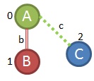
If we look back further in our algorithm we find that we also haven't checked all of the growth priorities off of the first frequent edge (0,1,A,b,B). Our first growth came from using the 3rd priority growth strategy, but we haven't checked the 4th/5th priority grown strategies there yet. If we do, we can see that it might be possible to make a link like (0,1,A,b,B) and (0,2,A,c,C). Let's see if we can find that in the graphs

We can see that in all four of our remaining graphs so we'll keep this sub-graph.
Our first priority for growth on this sub-graph would be to connect back to the root, but we don't have any double bonds (sorry for the chemistry reference) in our example so that won't work. The 2nd priority is also impossible, so let's check the 3rd. Can we grow an edge off of the C node? Our 2 options would be (2,3,C,a,B) and (2,3,C,c,A). Adding (2,3,C,a,B) looks like this.
When we search through the graphs, we find this in 2 places

Notice that I'm not counting the instances in the 2nd and 3rd graphs. This is because the only way you can get find this subgraph in those graphs is to wrap the graph such that the 1 B node is the same as the 3 B node. The reason why we number the nodes is to make sure they're unique, plus we already found the sub-graph that creates that ABC triangle previously...thus the beauty of the algorithm :). Since there are only 2 graphs with this sub-graph, the minimum support of 3 is not met.
So now let's check for the other growth option (2,3,C,c,A)
That can only be found in one of the graphs

So now we've exhausted our growth options off of the first edge (A,b,B).
2nd Edge (A,c,C)
Before you go crazy thinking that the other 2 edges we need to check will take just as long, let me tell you that we have already done WAY more than half of the work on this problem. Now that we have exhaustively checked all of the graphs for frequent sub-graphs that contain the edge (A,b,B), we can trim down our search space significantly. What I mean is we can delete edges in graphs that contain (A,b,B) and only look for frequent patterns in what is left. If we do this, we get 4 graphs (remember we already got rid of graph 5 because it contained no frequent edges) that look like this.
These graphs are much simpler. I also wanted to point out that I removed any edges from these graphs that were not frequent. We could (should) have done this earlier when we were doing our search on the first edge, but I didn't want to complicate things at that time. Now, much like last time, we start with edge (0,1,A,c,C) and try to grow from 'C'. We can either use (1,2,C,a,B) or (1,2,C,c,A). If we add (1,2,C,a,B) we can find that sub-graph in the following places

All 4 graphs have this sub-graphs, so it's a keeper and we'll go with it (remember we haven't checked adding (1,2,C,c,A) yet. The next step is to try to grow from the last vertex back to the root. If we did this we would have to use the edge (B,b,A), but that edge has been removed from all of our graphs because we have already mined all of the frequent sub-graphs with (A,b,B) in them. So, our only other growth option is to try to extend the chain from 'B'. The only option left to grow from 'B' is (B,a,C) because (B,b,A) has already been checked. So we get a sub-graph like this.

That's 3 out of the 4 graphs, which meets our support requirement so we'll keep it. Our first growth priority from here is to link node 3 ('C') back to the root. That would be adding a (3,0,C,_,A) link. The only link possible for this in our data set is (3,0,C,c,A) which would give us this subgraph to look for
The only place this subgraph is found is in our 2nd example:

However, that subgraph is only found here:

So, we back up again and try our 4th priority, which is growing a link off of the B at node 2. A quick look at the graphs above show that won't work. Lastly, we'll try to grow further up the graph, like a new node coming off the C at node 2 or a new node off the A at node 0. There's a couple options for growth off of node 2, but I can tell it's only supported by our first graph. There are no additional options for growth from the root node 'A'. so we're done exploring this graph branch.
Now we need to step back to when we had the graph (0,1,A,c,C), (1,2,C,a,B) and try to grow again from there. The last priority for growth for this subgraph is to grow from the root. The only way we can grow from the root is to add (A,c,c), which would look like this.
Since this is only found in one place, it's a dead end and we need to backtrack to other options we didn't pursue earlier. We only had one of those when we were adding our 2nd edge to (A,c,C). So when we go back and try to add (1,2,C,c,A) to (0,1,A,c,C) we look at our graphs and find that it is only present in 2 of our graphs
As it turns out these are all of our options starting with edge (A,c,C). See, I told you the 2nd edge would go faster than the first.
3rd Edge (B,a,C)
Now we have to check the last of our frequent edges to see if there is any way that we can grow a frequent sub-graph with just this edge. Let's start by removing all of the (A,c,C) edges from our graphs to see what we're left with.
I could go through all of the same procedure I have been using for these remaining graphs, but it gets so simple at this point that there really isn't a reason to. If you're using a program runing the gSpan algorithm, it will be disciplined and do the whole search though. From what is left, we can see that (0,1,B,a,C); (0,2,B,a,C) is frequent, but anything larger doesn't work out. We hit our last dead end and now we can report all of the sub-graphs that we found that were frequent.

I have them organized by the edge they were grown from. The last thing we have to do is translate our DFS codes back to the original symbols. This is easy enough and the user would get an output like this.


.jpg)