Showing posts with label Interesting. Show all posts

Tuesday, March 3, 2015

Null-Invariant Measures of Interestingness

In 2 of my previous posts about measures of interestingness (Lift and Chi-Square) I mentioned I would be writing a post about null-invariant measures of interestingness.  I'm a man of my word so here you go.  The problem I presented in those posts can be summarized with these 2 tables.


If you click back to those previous posts (links above) you'll see that the lift for the first table was 0.714 and the lift for the 2nd table would be calculated as 0.929.  The chi-square value for the first value was 0.586 and the value for the 2nd is calculated as 0.022.  For both these measures we get different numbers when the size of the bottom right cell ("null" count) is changed.  The table below shows this information in a slightly different view.


Since we're pattern mining, and we're really only interested in the interaction between the two items (apples and oranges in this example), we'd love to have a way to measure interestingness that doesn't include that "null" count in the calculation at all.  Data scientists call this type of an interestingness measure "null-invariant".  Let's see what they've come up with to help us out here.

Based on a white paper entitled "Selecting the Right Interestingness Measure for Association Patterns" written by Pang-Ning Tan, Vipin Kumar and Jaideep Srivastava in 2002, there are 3 measures for interestingness that have this "null-invariant" property that we're looking for.  The three that they found are Confidence, Cosine, and Jaccard.  The Confidence measure actually has at least 3 variations to it now that I'm aware of so we'll cover 5 different null-invariant measures in total here.

Confidence
If you've read my post about support and confidence, you may remember near the end that I mentioned that confidence gives different values based on the way it's calculated (e.g the confidence for Apples à Oranges may not be the same as the confidence for Oranges à Apples).  If that is the case, which one should you pick?  With so many potential patterns that can be found in data already, it is preferable for data scientists to find a way to combine these 2 options to get 1 answer instead of having to duplicate all of their results to show both sides of the same coin all the time.  To do this, they have taken the original confidence equation P(A|B), or P(B|A) depending on how you look at it, and created the following alternate forms

At this point in time it is my duty as your guide to understanding data mining in a simple way to calm you down if the stuff in the definition column gave you heart palpitations.  All three of these are actually VERY easy to understand if you already understand confidence.  I'm actually going to work from the bottom of this list up. Max Confidence basically says, I'm just going to pick the biggest value of confidence between the 2 ways of looking at it. Kulczynski (pronounced KƏl-zin’-skee) takes the approach of averaging the 2 together instead.  For, All Confidence, it may not be apparent, but you're actually taking the minimum value of confidence.  Since confidence is just the count (or support) of records that have both items (A∩B) divided by the count of the first item in a statement like AàB.  If you're dividing by the maximum value of the support for AàB and BàA, then you're really just finding the minimum value of confidence between the 2 options.  So, like I said, it might look scary, but it's simple.

Cosine
Another good interestingness measure is the cosine function.  The way that I think about the cosine function is that is essentially the lift function in disguise, but is null invariant.  Let me show you what I mean.  Here are the equations for both

You can see that the only real difference between the 2 is that Cosine has a square root in the denominator.  There's a good reason for this.  In my post about lift, I mentioned that to calculate lift correctly, you have to make sure you are using the support as a percent of the total records in the database.  If you don't do this, the lift value is wrong.  The fact that you have to divide by the grand total of all the records is also why the lift measure is susceptible to changes in the number of null records.  Cosine overcomes this with a trick I was taught in intermediate school

When I first saw the lift equation written out this way I really wanted to get the "grand total" values to cancel out because it would be so much cleaner.  Another way of writing (or think about) lift is something like this (AB/G)/((A*B)/G^2) where AB is the count of A & B together, A is the count of A, B is the count of B, and G represents the grand total.  Using fraction math, you can cancel out one of the grand totals, but not the 2nd one leaving you with (AB)/(A*B/G).  Cosine takes care of this problem.  When we take the square root of the denominator, we can cancel out the grand total from the function entirely making the measure null-invariant.  It looks like this: (AB/G)/sqrt((A*B)/G^2), which simplifies to AB/sqrt(A*B).

Jaccard
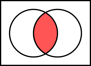
The Jaccard function is defined as |A∩B|/|A∪B|.  To explain what that means let's go to Venn diagram world.
As a reminder, that upside-down U symbol is an intersection and is represented by the orange area in the diagram above.  The right-side-up U symbol is a union and is represented by all of the area that is either yellow, orange or red.  The '|' symbols in the formula are just a notation that is used to indicate that we want the count of items in that set, instead of the set itself.  Now that that is fresh in our minds again, the numerator of the Jaccard is the Orange area, and the denominator is the area of the yellow-orange-red area, NOT double counting the orange area because of the perceived overlap.  With that understanding, you can see why Jaccard is null invariant; it doesn't use any data from the blank space, null records, to be calculated.  I could make the white space in Venn diagram above HUGE and the Jaccard would still have the same value. 

Comparisons
Lastly, let's take a look at our apple and orange example one more time with all of these different measures of interestingness.

First of all, in the 2nd row, you can see that all of the measures we've added to this table aren't affected by the different "null" number.  I also have added a couple of rows to demonstrate how the different measures change with different values in the table.  In row 3 you can see a what a positive correlation looks like, instead of a negative one.  In row 4, you can see what no correlation looks like.  It's interesting to note that for Jaccard no correlation is represented by a value of 1/3.  Then in rows 5 and 6 I showed the extremes of these null variant measures...all of them are bound between 0 and 1.  0 means STRONG negative correlation, and 1 means STRONG positive correlation.  

Row 7 is there as a tale of caution.  Based on an astute comment on this post, revised/change the table above so that you can compare rows 1, 2, and 3.  They all have the same values except for the "null" number.  If the "null" number gets too big, like in row 7, then "someone who has bought an orange is far more likely than the general population to buy an apple".  This is not immediately obvious, and can be a stumbling block when using null-invariant measures of interestingness.

I think that sums it up.  I hope that helps!

Saturday, February 28, 2015

Chi-Squared

Another method of "interestingness" that can be used in data mining is the chi-square test.  This test is actually one that I have a fair amount of experience with from my six sigma and manufacturing background.  I'll use a simple example from my past to walk you through how it is calculated first, then give some warnings about ways it can be misused.

Suppose you have a factory that makes widgets and have 2 machines in the manufacturing process that perform the same step, say they're both plastic injection molding machines.  When parts come out you have an inspector that classifies the parts as good or bad.  Over time, you collect all of this data and come up with a table like the one below.

I looks like they produced roughly the same quantity of bad parts, but machine 2 also made less parts overall.  What chi-squared will do is help us determine if that difference is (statistically) significant.  The first thing we need to do is determine what we would expect if the 2 machines had the same quality.  To get this expectation we use the values in the row total and column total.  If there were no real difference between the 2 then we would expect there to be a good ratio of 605/657=92.08% for both machines.  To get the bad ratio (defect rate) we just take 1 minus the good ratio and we get 7.92%.  Now we just need to account for the fact that the 2 machines produced different quantities.  With these expected good/bad ratios we can calculate how many good parts we expect if we produce 400 or 257 parts.  We would expect that machine 1 would produce 400*92.08% = 368.34 good parts and 400*7.92%=31.66 bad parts.  We would expect that machine 2 would make 257*92.08% = 236.66 good parts and 257*7.92% = 20.34 bad parts.  this gives us an expected table that looks like this.

The formula to calculate any expected value in the table above is [Row Total]*[Column Total]/[Grand Total].  If you look back to the logic in the paragraph above, you'll see that is exactly what we did.

Now that we have expected values, we can calculate the chi-square statistic.  This is done by taking each cell (e.g. good parts from machine 1 as one example) and calculate (observed value - expected value)^2/(expected value).  For the upper left cell this would be (375-368.34)^2/368.34 = 0.1203.  After doing this for each cell we get a table that looks like this.

Then you just have to add these up to get you your chi-square statistic; in this example it's 3.89.  A chi-square statistic doesn't mean much unless you know how many degrees of freedom you have.  Don't know what degrees of freedom means?  That's OK.  For now, all you need to know is that for a chi-square test it is equal to (# of rows - 1)*(# of columns - 1).  We just have a 2x2 table here so we get (2-1)*(2-1) = 1 degree of freedom.  The 3.89 chi-squared value and the 1 degree of freedom are used to lookup a p-value. I think of a p-value as a probability value.  When you're looking at a p-value, you are looking at the expected probability that nothing interesting is going on in your data.  So, if you want to find something interesting, you're hoping for REALLY small p-values.  In order to get the p-value I almost always use MS Excel.  The Excel function would look like this "=CHIDIST(3.89,1)".  For our problem, we get a p-value of 0.0486.  This can be interpreted that we think there is 4.86% chance that nothing interesting is happening here.  A common threshold that statisticians use for this p-value is 5%.  Since, our 4.86% is less than 5%, we would say that this difference is statistically significant.  

Now that we know the mechanics of how to calculate it, let's talk briefly about the intuition behind the numbers.  If 2 features (e.g. good/bad and machine 1/2) have nothing interesting going on what is the chi-square value going to be?  To start, you would expect the values in the expectations table to be exactly the same as the data you started with. Once you know that, you also know that all of the values in the chi-square table will be zero; (observed-expected)^2/expected will give you 0 divided by something, which is zero.  The chi-square value can never be negative because the numerator is a squared value, and the denominator is an expected number of positive counts.  The least interesting thing possible is 0, and the most interesting thing would be...some ridiculously large number (theoretically infinity), but in real life you don't ever get infinity as the answer.

Now, after all that explanation, I've got to let you down a little bit because chi-square isn't very good for data mining applications for the same reason why the lift measure has problems.  If we use the same example that I used in my lift post, we have transactions for apples and oranges like this


If I follow the instructions above to calculate chi-square for the first table, I get 0.586.  If I do the same thing for the 2nd table, I get 714,283.7...hmmm.  In theory the interaction between apple and orange purchases are the same in both tables, but the chi-square statistic gets very confused by the double null transactions.  That is why null-invariant measures for interestingness are so important when mining data patterns (another post to come soon explaining these measures).


Thursday, February 26, 2015

Lift

Lift is an objective measure of "interestingness" that has been used in various fields including statistics.  It is also an option when we are data mining.  In case you've run across this measure and don't fully understand it, let me give you a quick summary of what it is, how it's calculated and some of its properties.

Much like the properties of support and confidence, lift attempts to use a numerical calculation to determine how importance a pattern or correlation is.  If we use the table below as a simple example we can kind of see that people who buy oranges, are less likely to buy an apple and vice versa (this is called a negative correlation), but in a data mining process we want to have an automated way to see this.  Lift is one option to automate and determine this.


To calculate lift, first find the support for both items together (in this case 2/20=10%.) and this will be your numerator.  Notice that I used the "% of total" version of support.  If you don't do this you will get a different answer and it will be wrong.  For the denominator, multiply the total support for both items together (bottom left and top right total values); in this case that would be 8/20 * 7/20 = 0.14.  The lift for buying apples and oranges together would be ~0.714 for this example.

So what does this 0.714 mean really?  If, the lift were to work out to equal exactly 1, then that would mean that there is no correlation at all between the 2 items.  Since, our lift is less than 1, it means that there is a negative correlation (that's what we could see with our own intuition before we started).  If the lift turns out to be greater than 1, then there is a positive correlation.  If you look at how lift is calculated you will notice that because all of the values that go into the fraction are positive counts (or fractions of positive counts), the value of lift always has to be positive (>0).  It can get really BIG though.  If I change the table above to have lots of transactions without apples or oranges, then I can get a really big number for my lift

If you do the same calculation we did above on this table, you get a lift of 357,143.32. This huge swing in the lift value is the greatest limitation of lift in data mining.  The only thing I changed in the data I was analyzing was the number of transactions that didn't have apples or oranges.  Intuitively this shouldn't make any difference whether the correlation is interesting or not.  That is why data mining has developed other measures of interestingness that are called null-invariant.  Null-invariant measures aren't sensitive to that lower right value in the table.  Eventually I'll write a blog post about those and add a link here, but that won't be tonight.


Thursday, February 12, 2015

Support and Confidence in Pattern Discovery

When analyzing patterns in data, what we are really looking for are patterns that are interesting.  There are subjective ways to determine if data is interesting, but data analysis can be sped up significantly by creating objective measures for "interesting".  When looking for patterns, associations and correlations in data, many algorithms will use the objective measures of support and confidence.  These concepts are easier to understand looking at an example.


Example: Suppose we have happen to have a small sample of the transaction records from a grocery store.  The transactions might look something like this:


A quick glance at this table shows that there seems to be a pattern of buying milk at the same time bread is bought, but let's figure out what the support and confidence for this is.  The support for a pattern between milk and bread are the instances where they show up together in a transaction.


Basically this is the equivalent of an AND logic statement.  So, for our example above the support for Milk U Bread would be 3.  In larger datasets, it makes more sense to divide this number by the total number of transactions so we can get a feeling for what percentage of transactions have these items together.  If we did that the support would be 60%.  Support does not have to be just for 2 items, we can figure out support for 1 item alone (support for Salsa = 1, or 20%) or for several items together (support for Flour, Milk and Bread = 1,or 20%)


Confidence is defined as P(Y|X).  If it's been a couple years since you were in a statistics class, that probably when over you head, but that's OK...don't be afraid. In math speak P(Y|X) means "probability of Y given X".  In English it means, if you already know that you have something, say milk = X, in your transaction, then what's the probability that you also have something else, say bread = Y?  So if you have milk...
What percentage of the transactions that have milk have bread also?
So to calculate the Confidence that if you have milk, you have bread too, just take the support for milk and bread (we counted 3 above) and divide it by the support for milk (it's 4 in our list).  That gives a confidence of 75%.  The mathematical notation for this association is Milk --> Bread (60%, 75%).  The 60% is the support for the pair pattern, and the 75% is the confidence.  Notice that this calculation can be done both ways.  What if I know I have bread and want to know the confidence I have of there being milk also?  The support for the combination of the two items is still 3, but the support for bread on its own is also 3.  That means the confidence is 100% based on our data.  So Bread --> Milk (60%, 100%).  It's obvious from the numerical results that the Venn diagrams I drew above are definitely NOT to scale, but it makes it easier to visualize the difference between the different items and their intersection.