Saturday, February 28, 2015

Chi-Squared

Another method of "interestingness" that can be used in data mining is the chi-square test.  This test is actually one that I have a fair amount of experience with from my six sigma and manufacturing background.  I'll use a simple example from my past to walk you through how it is calculated first, then give some warnings about ways it can be misused.

Suppose you have a factory that makes widgets and have 2 machines in the manufacturing process that perform the same step, say they're both plastic injection molding machines.  When parts come out you have an inspector that classifies the parts as good or bad.  Over time, you collect all of this data and come up with a table like the one below.

I looks like they produced roughly the same quantity of bad parts, but machine 2 also made less parts overall.  What chi-squared will do is help us determine if that difference is (statistically) significant.  The first thing we need to do is determine what we would expect if the 2 machines had the same quality.  To get this expectation we use the values in the row total and column total.  If there were no real difference between the 2 then we would expect there to be a good ratio of 605/657=92.08% for both machines.  To get the bad ratio (defect rate) we just take 1 minus the good ratio and we get 7.92%.  Now we just need to account for the fact that the 2 machines produced different quantities.  With these expected good/bad ratios we can calculate how many good parts we expect if we produce 400 or 257 parts.  We would expect that machine 1 would produce 400*92.08% = 368.34 good parts and 400*7.92%=31.66 bad parts.  We would expect that machine 2 would make 257*92.08% = 236.66 good parts and 257*7.92% = 20.34 bad parts.  this gives us an expected table that looks like this.

The formula to calculate any expected value in the table above is [Row Total]*[Column Total]/[Grand Total].  If you look back to the logic in the paragraph above, you'll see that is exactly what we did.

Now that we have expected values, we can calculate the chi-square statistic.  This is done by taking each cell (e.g. good parts from machine 1 as one example) and calculate (observed value - expected value)^2/(expected value).  For the upper left cell this would be (375-368.34)^2/368.34 = 0.1203.  After doing this for each cell we get a table that looks like this.

Then you just have to add these up to get you your chi-square statistic; in this example it's 3.89.  A chi-square statistic doesn't mean much unless you know how many degrees of freedom you have.  Don't know what degrees of freedom means?  That's OK.  For now, all you need to know is that for a chi-square test it is equal to (# of rows - 1)*(# of columns - 1).  We just have a 2x2 table here so we get (2-1)*(2-1) = 1 degree of freedom.  The 3.89 chi-squared value and the 1 degree of freedom are used to lookup a p-value. I think of a p-value as a probability value.  When you're looking at a p-value, you are looking at the expected probability that nothing interesting is going on in your data.  So, if you want to find something interesting, you're hoping for REALLY small p-values.  In order to get the p-value I almost always use MS Excel.  The Excel function would look like this "=CHIDIST(3.89,1)".  For our problem, we get a p-value of 0.0486.  This can be interpreted that we think there is 4.86% chance that nothing interesting is happening here.  A common threshold that statisticians use for this p-value is 5%.  Since, our 4.86% is less than 5%, we would say that this difference is statistically significant.  

Now that we know the mechanics of how to calculate it, let's talk briefly about the intuition behind the numbers.  If 2 features (e.g. good/bad and machine 1/2) have nothing interesting going on what is the chi-square value going to be?  To start, you would expect the values in the expectations table to be exactly the same as the data you started with. Once you know that, you also know that all of the values in the chi-square table will be zero; (observed-expected)^2/expected will give you 0 divided by something, which is zero.  The chi-square value can never be negative because the numerator is a squared value, and the denominator is an expected number of positive counts.  The least interesting thing possible is 0, and the most interesting thing would be...some ridiculously large number (theoretically infinity), but in real life you don't ever get infinity as the answer.

Now, after all that explanation, I've got to let you down a little bit because chi-square isn't very good for data mining applications for the same reason why the lift measure has problems.  If we use the same example that I used in my lift post, we have transactions for apples and oranges like this


If I follow the instructions above to calculate chi-square for the first table, I get 0.586.  If I do the same thing for the 2nd table, I get 714,283.7...hmmm.  In theory the interaction between apple and orange purchases are the same in both tables, but the chi-square statistic gets very confused by the double null transactions.  That is why null-invariant measures for interestingness are so important when mining data patterns (another post to come soon explaining these measures).


Thursday, February 26, 2015

Lift

Lift is an objective measure of "interestingness" that has been used in various fields including statistics.  It is also an option when we are data mining.  In case you've run across this measure and don't fully understand it, let me give you a quick summary of what it is, how it's calculated and some of its properties.

Much like the properties of support and confidence, lift attempts to use a numerical calculation to determine how importance a pattern or correlation is.  If we use the table below as a simple example we can kind of see that people who buy oranges, are less likely to buy an apple and vice versa (this is called a negative correlation), but in a data mining process we want to have an automated way to see this.  Lift is one option to automate and determine this.


To calculate lift, first find the support for both items together (in this case 2/20=10%.) and this will be your numerator.  Notice that I used the "% of total" version of support.  If you don't do this you will get a different answer and it will be wrong.  For the denominator, multiply the total support for both items together (bottom left and top right total values); in this case that would be 8/20 * 7/20 = 0.14.  The lift for buying apples and oranges together would be ~0.714 for this example.

So what does this 0.714 mean really?  If, the lift were to work out to equal exactly 1, then that would mean that there is no correlation at all between the 2 items.  Since, our lift is less than 1, it means that there is a negative correlation (that's what we could see with our own intuition before we started).  If the lift turns out to be greater than 1, then there is a positive correlation.  If you look at how lift is calculated you will notice that because all of the values that go into the fraction are positive counts (or fractions of positive counts), the value of lift always has to be positive (>0).  It can get really BIG though.  If I change the table above to have lots of transactions without apples or oranges, then I can get a really big number for my lift

If you do the same calculation we did above on this table, you get a lift of 357,143.32. This huge swing in the lift value is the greatest limitation of lift in data mining.  The only thing I changed in the data I was analyzing was the number of transactions that didn't have apples or oranges.  Intuitively this shouldn't make any difference whether the correlation is interesting or not.  That is why data mining has developed other measures of interestingness that are called null-invariant.  Null-invariant measures aren't sensitive to that lower right value in the table.  Eventually I'll write a blog post about those and add a link here, but that won't be tonight.


Tuesday, February 24, 2015

Core Patterns of Colossal Patterns


Professor Jiawei Han at the University of Illinois and some of his colleagues created a method of data mining to find what are called colossal patterns.  "Colossal" in this context basically means really big patterns with lots of different items included.  As an example of this, think about people working in biostatistics looking for large sequences of DNA that are interesting.  The "Pattern-Fusion" method that they created has 2 parts to the algorithm.
  1. Use a regular pattern generation method (e.g. Apriori, FP Growth, etc.) to create the first couple levels of patterns that are supported.  A common level of complexity for this step to  stop is when the algorithm has 3-item patterns (e.g. ABC), but this can be selected by the user when this algorithm is run
  2. Take these large-ish patterns and combine them together to make bigger patterns faster than incrementally looking for patterns that only have 1 more item.
The reason why this method is so valuable can be seen if you look at how many possible combinations(patterns) are possible as the number of items increases.  The table below shows the number of combinations possible if you have 5, 10, or 15 items in each column, and pick 1-15 items in the rows.

If you're really only interested in finding the BIG patterns that the data supports, you don't really want to get bogged down in looking at 6,435 patterns that have 7 items in them (see the last column above).  Plus, this tabular example above is VERY simplified, how many sequences are in a strand of DNA?  Oh yeah! Old algorithms might get bogged down forever in that mess in the middle for that type of problem. 


Core Pattern and Pattern Robustness
Now that I've summarized the conceptual process, I'm going to explain core patterns and pattern robustness.  Core patterns are the ones that the algorithm "likes" to use in order to create the BIG patterns it's really looking for.  I got my butt kicked by these 2 concepts during my quiz for professor Han's Coursera course, so I figured I should probably take the time to really understand them and explain them simply for everybody else.


In Han's textbook, Data mining : concepts and techniques, he says that...
"for a pattern α, an itemset βα is said to be a t-core pattern of α if  where  is the number of patterns containing α in database D." emphasis added.

Say what?!? For those of you out there who are not fluent in mathspeak, I will translate.  For a pattern named Beta to be a core pattern of pattern Alpha it needs to meet a couple requirements.

Criteria 1
Beta needs to be a subset of Alpha (βα).  In Venn diagram world this looks like the diagrams below. The line under that 'c' looking symbol means that β can actually be as big as α (kind of like a less-than-or-equal-to symbol), and therefore they can be the same set of items and still satisfy this criteria.


Criteria 2

That complicated equation needs to have a value greater than τ.  What is tau, other than a greek letter?  It' just a value between 0 and 1 that the user of the algorithm picks so that there is a criteria to rate patterns against.  If the calculated value in the equation is really high, we're more certain the pattern being considered is a core pattern, if it's really low...not so much.  That explains tau, but now we need to understand the equation.

|Dα| is defined as "the number of patterns containing α in database D".  Although the symbols might be confusing, this is actually relatively easy to calculate.  Just count up all of the records, transactions, etc. in your database that have the pattern α.  You need to make sure that your looking at sub-patterns too.  Say one transaction has ABDFE, and you're looking for ABF (this is α in this example), this transaction counts for this calculation.  The same process is followed for β but based on the first criteria, β is going to be a smaller subset pattern of α or the same pattern as α.  So in the quick example above, β might be A, AB, AF, BF, or even ABF.  The whole point of this ratio is to give a measure for how important β is in the make-up of the bigger pattern α.  If there are 100 records that contain α, and 250 records that contain β, then this core pattern "strength", as I'll call it, would be 0.4 (P.S. don't get confused by the Venn diagrams above here.  Those diagrams are for the items in the patterns themselves, NOT for the frequency of the patterns in the database you're mining).  If tau were set by the user as 0.25, then β would be considered a .25-core pattern of α.

Example
Now let's use an example to clarify this and show how to calculate core pattern robustness.  Suppose we have a database with some patterns that have the counts as shown in the table below
Let's assume that we set tau to be equal to 0.5.  So we'll need to do the core pattern calculation explained above for all of the subsets of each item in this list to see if they are a core pattern.  For the first pattern, ACE, there are 10 instances in the database (this one is simple, but others are a little tricky).  Now we figure out the counts for A, C, E, AC, AE, and CE in the database.  A=20, C=40, E=10, AC=20, AE=10, CE=10, and we already know ACE=10.  So, for each of these patterns we can calculate the ratio ACE/A=0.5; ACE/C=0.25; ACE/E=1; ACE/AC=0.5; ACE/AE=1; ACE/CE=1; and ACE/ACE=1.  So based on our criteria, tau = 0.5, we have core patterns of A, E, AC, AE, CE, and ACE; C got cut out because it only had 0.25.

BCD on the next line is similar, but for BCD the count is 20 because BCD has 10 transactions in the 2nd row and 10 transactions in ABCDF in the 4th row; told you there were trickier ones.  Follow the same process as the above paragraph for the rest of the calculations. If you do this, you should come up with a table that looks something like this.  

As an exercise, try to figure out which patterns didn't make the cut.  There are three of them, and I already showed you one of them already.  Obviously if the value of tau were set lower, we would have cut out a lot more patterns and the table would have a lot fewer entries in the last column

Core Pattern Robustness
Now, we need to explain pattern robustness.  if you have the information above already, pattern robustness is pretty easy to figure out.  In mathspeak, and example of how robustness might be stated goes something like this "A pattern α is (d, τ) robust if d is the maximum number of items that can be removed from α for the resulting pattern to remain a τ-core pattern." (Han's textbook again).  All that really means is that you're trying to answer the question, "how many items can I remove from the pattern I'm looking at and still have what's leftover qualify as a core pattern?".  For the first pattern in the table above, ACE, we have 3 items A, C, and E.  If we take away 1 item, say A, we can see that CE is still a core pattern in the table.  if we take away a 2nd item C, E is still a core pattern.  If we took away E, we'd have nothing so that's no good.  By definition the null set, or nothing, can't be a core pattern.  So for ACE we were able to take away 2 items and still have a core pattern.  So, if we were to translate that example to mathspeak we would be able to say that pattern ACE is (2, 0.5)-robust.  Using similar logic we could add another column to our table stating robustness of each of the rows.  Please double check me...at the time of this writing it is getting late and my mental powers are waning. :)

I hope this helps people out there understand something that took me quite a while to understand from just a couple of sentences in a textbook.


Tuesday, February 17, 2015

Closed Itemsets

When we are looking for patterns in data sets, often the amount of patterns that can be found can be huge.  To demonstrate this I'll use a simple set of examples.  Lets say that you have one transaction with items A and B (I know this wouldn't give you much information, but it proves my point).  In this transaction there are 3 patterns/combinations: A, B and AB.  Now let's say that the transaction has A, B, and C in it.  This transaction allows for 7 patterns: A, B, C, AB, AC, BC, and ABC.  If it had A, B, C, D, then there would be 15 patterns: A, B, C, D, AB, AC, AD, BC, BD, CD, ABC, ABD, ACD, BCD, and ABCD. You can see that the number of patterns that can be created grows MUCH faster than the number of items in the transaction. This growth pattern is based on the mathematical concept of combinations (wikipedia).

Also, any data set that anybody would actually care about would have more than one transaction, probably thousands, if not millions or billions.  This explosion of complexity that comes from all of the possible patterns that can be found in data is the motivation for ways of compressing the possible patterns/combinations.  That is what closed itemsets are all about.

CLOSED ITEMSETS

Now I'm going to have to get a little technical here, but I'm going to translate for you too so don't worry.  The definition of a closed pattern goes like this, "A pattern (itemset) X is closed if X is frequent, and there exists no super-pattern Y  X, with the same support as X" (J. Han, Pattern Discovery in Data Mining, Coursera Lecture Material) 

Let's break this definition down.  "itemset" is just a group of items.  It could be one item (A), 2 items (AB), 3-items (ABC)... k-items. People sometimes refer to itemset size by telling you what k equals.  k is just a variable that represents the size/complexity of the pattern you're looking at. By, "frequent", the definition is saying that this itemset, X,  you're looking at meets the minimum support requirements, so it might be interesting.  The whole bit in the definition about "super-pattern Y  X" Basically means that all of X is contained in Y.  In Venn diagram world, if Y is a super-pattern of X then it looks like this

supper-pattern Venn diagram

In our example above, an example of this "super-pattern" notion would be like saying that ABC is a super-pattern of AB.  The notation Y  X is a fancy mathematical way of saying the same thing. The way I think about a closed pattern is that it's the biggest, most complex, pattern I can find at various levels of support.  It isn't exactly like that, but it will become clearer with an example.

Let's suppose we have a simple set of transactions like this
Simple transaction table

If you are looking for patterns that have support greater than or equal to 1, there would be a lot of combinations possible for just 2 transactions.  Based on the work we already did above, there are 15 combinations for the first transaction.  Transaction 20 also has the 15 combinations, but there is some overlap in possible combinations in transaction 10 and 20.  To visualize this, lets list them out in a table.


Combination Table

 If you look closely at the combination table above, you can find some repeats if you compare transaction 10 and 20.  To make this easier to see, I've rearranged the entries a little bit here.


Expanded Combination Table

The green highlighted combinations are found in both transactions.  Based on this, there is support of 1 for every combination in the expanded combination table, except for C, D, and CD which have support of 2.  This is where closed itemsets come in handy.  If you remember the Apriori Principle, if a more complex combination meets the minimum support requirements, then the subset, or simpler patterns, will also meet those requirements.  In this example, if I make the statement that I know that CD has support of 2, then I automatically know that C, and D also have support of at least 2.  In this case C and D have a support of exactly 2 so CD is one of my closed patterns in this data.  Let's revisit the definition of a closed pattern to make sure that's true.  There are 2 requirement for a pattern to be a closed pattern
  1. It's frequent; yep CD meets that criteria
  2. No super-pattern with the same support as CD;  There are bigger patterns in the data, but none of them have support of 2 so we're good here too
What's so awesome about this is that I can say I have closed pattern CD with support of 2, and I automatically know that C and D also have support of 2 because of the apriori principle.  We can use this one close pattern to compress three patterns without losing any information!

Now let's look for some other closed patterns in the data, so you can get the hang of it.  The way I explained closed data sets before was that they are normally the most complicated patterns that are frequent.  In our table above we've got ABCD and CDEF to work with that seem to fit that criteria.  So which one is a closed pattern? Both actually.  Let's look at the 2 rules for ABCD

  1. It's frequent; in our example we only need frequency of 1, so we're good here
  2. No super-pattern with the same support as ABCD;  CDEF has the same support as ABCD, but CDEF is not a supper pattern of ABCD.  
The same logic is applied to CDEF.  Going back to Venn diagram world the whole set of closed patterns in this data looks like this, where S is the support for each closed pattern.
Closed pattern Venn diagram

If you use the Apriori principle, and these 3 closed patterns, you can reconstruct the entire data table we started with without losing any information.  Pretty awesome right?

MAX-PATTERN ITEMSETS

There is another way to compress pattern data called max-patterns.  They are almost exactly the same as closed patterns, except that we don't care about whether other patterns have the same support.  A max-pattern still has to satisfy the minimum support threshold though.  The easiest way to explain this is by using the example above for closed patterns.  In that example we have closed patterns ABCD, CD, and CDEF. CD is a distinct closed pattern because it has a support of 2 and the others only have support of 1.  This is despite that fact that it is actually a subset, or part of, ABCD and CDEF.  If you're looking for max-patterns you don't care about this distinction so you only get ABCD and CDEF as max-patterns; that's because CD is part of the larger patterns ABCD and/or CDEF.  A max-pattern will give you more pattern compression, but you can see that even in this very simple example, you're losing some of the information that was originally contained in the raw data because now we don't know how much support CD, C, or D had.


Apriori Principle


When making sure that all of the patterns in a set of data meet the minimum support requirements, we want to find all of the patterns that are supported, and not waste time looking at patterns that aren't.  This seems simple, but in much larger data sets, it can become difficult to keep track of which patterns are support and which aren't.  The Apriori Principle helps with this.

To explain, let's use the data in this table and assume that the minimum support is 2.


We start by looking for single items that meet the support threshold.  In this case, it's simply A, B, C, D, and E, because there is at least 2 of each of these in the table.  This is summarized in the single item support table below

single item support table

Next, we take all of the items that meet the support requirements, everything so far in this example, an make all of the patterns/combinations we can out of them; AB, AC, AD, AE, BC, BD, BE, CD, CE, DE.  When we list all of these combinations in a table, and determine the support for each, we get a table that looks like this.
2 items support before filtering

Several of these patterns don't meet the support threshold of 2, so we remove them from the list of options.
2 item support table

At this point, we use the surviving items to make other patterns that contain 3 items.  If you logically work through all of the options you'll get a list like this: ABC, ABD, ABE, BCD, BCE, BDE (Notice that I didn't list ABCD, or BCDE here because they are 4 items long).


Before I create the support table for these let's look at these patterns.  The first one, ABC, was created by combining AB and BC.  If you look in the 2 item support table (before or after filtering), you'll find that AC doesn't have the minimum support required.  If AC isn't supported, a more complicated pattern that includes AC (ABC) can't be supported either.  This is a key point of the Apriori Principle.  So, without having to go back to the original data, we can exclude some of the 3-item patterns.  When we do this, we eliminate ABC (AC not supported), ABD (AD not supported), ABE (AE not supported), BCE (CE not supported) and BDE (DE not supported).  This process of removing patterns that can't be supported because their subsets (or shorter combination) aren't supported is called pruning.  This pruning process leaves only BCD with a support of 2.

3 item support table

The final list of all of the patterns that have support greater than or equal to 2 are summarized here.


Takeaways:
  1. The Apriori Principle can be used to simplify the pattern generation process when mining patterns in data sets
  2.  If a simple pattern is not supported, then a more complicated one with that simple pattern in it can not be supported (e.g. if AC isn't supported, there is no way that ABC is supported)
  3. You can also look at takeaway 2 in the opposite direction. If a complicated pattern meets the minimum support requirements, all of the simpler patterns that can be created from that complicated pattern must be supported. (e.g. if ABC is supported, then AB, BC, AC, A, B, and C all have to be supported)

Thursday, February 12, 2015

Support and Confidence in Pattern Discovery

When analyzing patterns in data, what we are really looking for are patterns that are interesting.  There are subjective ways to determine if data is interesting, but data analysis can be sped up significantly by creating objective measures for "interesting".  When looking for patterns, associations and correlations in data, many algorithms will use the objective measures of support and confidence.  These concepts are easier to understand looking at an example.


Example: Suppose we have happen to have a small sample of the transaction records from a grocery store.  The transactions might look something like this:


A quick glance at this table shows that there seems to be a pattern of buying milk at the same time bread is bought, but let's figure out what the support and confidence for this is.  The support for a pattern between milk and bread are the instances where they show up together in a transaction.


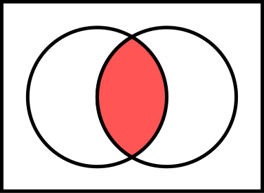
Basically this is the equivalent of an AND logic statement.  So, for our example above the support for Milk U Bread would be 3.  In larger datasets, it makes more sense to divide this number by the total number of transactions so we can get a feeling for what percentage of transactions have these items together.  If we did that the support would be 60%.  Support does not have to be just for 2 items, we can figure out support for 1 item alone (support for Salsa = 1, or 20%) or for several items together (support for Flour, Milk and Bread = 1,or 20%)


Confidence is defined as P(Y|X).  If it's been a couple years since you were in a statistics class, that probably when over you head, but that's OK...don't be afraid. In math speak P(Y|X) means "probability of Y given X".  In English it means, if you already know that you have something, say milk = X, in your transaction, then what's the probability that you also have something else, say bread = Y?  So if you have milk...
What percentage of the transactions that have milk have bread also?
So to calculate the Confidence that if you have milk, you have bread too, just take the support for milk and bread (we counted 3 above) and divide it by the support for milk (it's 4 in our list).  That gives a confidence of 75%.  The mathematical notation for this association is Milk --> Bread (60%, 75%).  The 60% is the support for the pair pattern, and the 75% is the confidence.  Notice that this calculation can be done both ways.  What if I know I have bread and want to know the confidence I have of there being milk also?  The support for the combination of the two items is still 3, but the support for bread on its own is also 3.  That means the confidence is 100% based on our data.  So Bread --> Milk (60%, 100%).  It's obvious from the numerical results that the Venn diagrams I drew above are definitely NOT to scale, but it makes it easier to visualize the difference between the different items and their intersection.